前言
最近几天都在阅读哈佛pytorch实现transformer的代码,代码风格很好,很值得参考和研读。和实验室师兄又在一起讨论了几次,代码思路和实现过程基本都了解了,对于原论文 “Attention is All You Need” 中关于transformer模型的理解又深入了许多。要想了解模型,还是要好好研读实现代码。以便于后面自己结合模型的研究。
本篇是对实现代码的注释,加上了自己的理解,也会有一些函数的介绍扩充。
参考链接
解读的是哈佛的一篇transformer的pytorch版本实现
http://nlp.seas.harvard.edu/2018/04/03/attention.html
参考另一篇博客
http://fancyerii.github.io/2019/03/09/transformer-codes/
Transformer注解及PyTorch实现(上)
https://www.jiqizhixin.com/articles/2018-11-06-10
Transformer注解及PyTorch实现(下)
https://www.jiqizhixin.com/articles/2018-11-06-18
训练过程中的 Mask实现
https://www.cnblogs.com/wevolf/p/12484972.html
transformer综述
https://libertydream.github.io/2020/05/03/Transformer-%E7%BB%BC%E8%BF%B0/
The Annotated Transformer
1 | # !pip install http://download.pytorch.org/whl/cu80/torch-0.3.0.post4-cp36-cp36m-linux_x86_64.whl numpy matplotlib spacy torchtext seaborn |
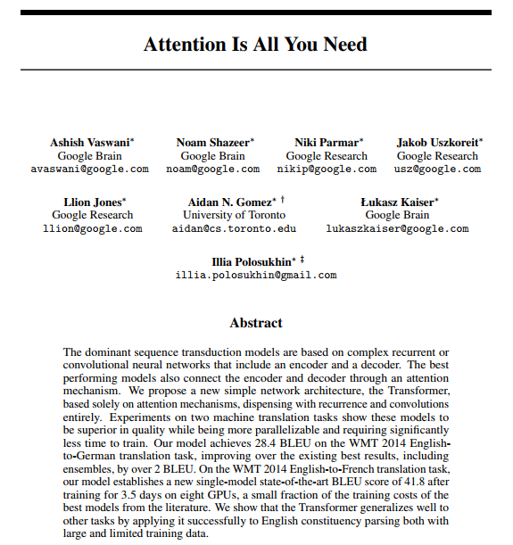
Transformer使用了Self-Attention机制,它在编码每一词的时候都能够注意(attend to)整个句子,从而可以解决长距离依赖的问题,同时计算Self-Attention可以用矩阵乘法一次计算所有的时刻,因此可以充分利用计算资源(CPU/GPU上的矩阵运算都是充分优化和高度并行的)。
模型结构
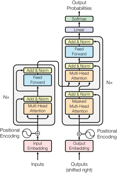
Most competitive neural sequence transduction models have an encoder-decoder structure (cite). Here, the encoder maps an input sequence of symbol representations(x1,…,xn) to a sequence of continuous representations z=(z1,…,zn). Given z, the decoder then generates an output sequence (y1,…,ym) of symbols one element at a time. At each step the model is auto-regressive (cite), consuming the previously generated symbols as additional input when generating the next.
EncoderDecoder定义了一种通用的Encoder-Decoder架构,具体的Encoder、Decoder、src_embed、target_embed和generator都是构造函数传入的参数。这样我们做实验更换不同的组件就会更加方便。
1 | class EncoderDecoder(nn.Module): #定义的是整个模型 ,不包括generator |
注:Generator返回的是softmax的log值。在PyTorch里为了计算交叉熵损失,有两种方法。第一种方法是使用nn.CrossEntropyLoss(),一种是使用NLLLoss()。很多开源代码里第二种更常见
The Transformer follows this overall architecture using stacked self-attention and point-wise, fully connected layers for both the encoder and decoder, shown in the left and right halves of Figure 1, respectively.
Encoder and Decoder Stacks
Encoder
Encoder和Decoder都是由N个相同结构的Layer堆积(stack)而成。因此我们首先定义clones函数,用于克隆相同的SubLayer。
这里使用了nn.ModuleList,ModuleList就像一个普通的Python的List,我们可以使用下标来访问它,它的好处是传入的ModuleList的所有Module都会注册到PyTorch里,这样Optimizer就能找到这里面的参数,从而能够用梯度下降更新这些参数。但是nn.ModuleList并不是Module(的子类),因此它没有forward等方法,我们通常把它放到某个Module里。
1 | def clones(module, N): #克隆N层,是个层数的列表。 copy.deepcopy是深复制, 一个改变不会影响另一个 |
1 | class Encoder(nn.Module): #定义编码器 |
1 | class LayerNorm(nn.Module): #norm部分 作为每一个子层的输出 |
不管是Self-Attention还是全连接层,都首先是LayerNorm,然后是Self-Attention/Dense,然后是Dropout,最后是残差连接。这里面有很多可以重用的代码,我们把它封装成SublayerConnection。
That is, the output of each sub-layer is LayerNorm(x+Sublayer(x)), where Sublayer(x) is the function implemented by the sub-layer itself. We apply dropout (cite) to the output of each sub-layer, before it is added to the sub-layer input and normalized.
To facilitate these residual connections, all sub-layers in the model, as well as the embedding layers, produce outputs of dimension dmodel=512.
1 | class SublayerConnection(nn.Module): # 每一个编码层中的两个子层 |
这个类会构造LayerNorm和Dropout,但是Self-Attention或者Dense并不在这里构造,还是放在了EncoderLayer里,在forward的时候由EncoderLayer传入。这样的好处是更加通用,比如Decoder也是类似的需要在Self-Attention、Attention或者Dense前面后加上LayerNorm和Dropout以及残差连接,我们就可以复用代码。但是这里要求传入的sublayer可以使用一个参数来调用的函数(或者有__call__)。
forward调用sublayer[0] (这是SublayerConnection对象)的__call__方法,最终会调到它的forward方法,而这个方法需要两个参数,一个是输入Tensor,一个是一个callable,并且这个callable可以用一个参数来调用。而self_attn函数需要4个参数(Query的输入,Key的输入,Value的输入和Mask),因此这里我们使用lambda的技巧把它变成一个参数x的函数(mask可以看成已知的数)。
Callable 类型是可以被执行调用操作的类型。包含自定义函数等。自定义的函数比如使用def、lambda所定义的函数
1 |
|
Decoder
The decoder is also composed of a stack of N=6 identical layers.
1 | class Decoder(nn.Module): |
1 | class DecoderLayer(nn.Module): #每一层解码层 |
src-attn和self-attn的实现是一样的,只不过使用的Query,Key和Value的输入不同。普通的Attention(src-attn)的Query是下层输入进来的(来自self-attn的输出),Key和Value是Encoder最后一层的输出memory;而Self-Attention的Query,Key和Value都是来自下层输入进来的。
Decoder和Encoder有一个关键的不同:Decoder在解码第t个时刻的时候只能使用1…t时刻的输入,而不能使用t+1时刻及其之后的输入。因此我们需要一个函数来产生一个Mask矩阵,所以代码如下:
注意: t时刻包括t时刻的输入
1 | def subsequent_mask(size): #将i后面的mask掉 |
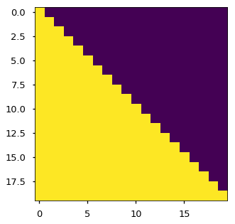
它的输出:
1 | print(subsequent_mask(5)) |
我们发现它输出的是一个方阵,对角线和下面都是1。第一行只有第一列是1,它的意思是时刻1只能attend to输入1,第三行说明时刻3可以attend to {1,2,3}而不能attend to{4,5}的输入,因为在真正Decoder的时候这是属于Future的信息。代码首先使用triu产生一个上三角阵:
1 | 0 1 1 1 1 |
然后需要把0变成1,把1变成0,这可以使用 matrix == 0来实现。
因为:布尔值True被索引求值为1,而False就等于0。
Attention
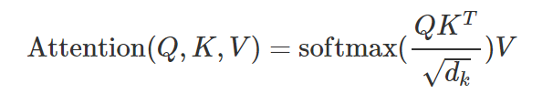
An attention function can be described as mapping a query and a set of key-value pairs to an output, where the query, keys, values, and output are all vectors. The output is computed as a weighted sum of the values, where the weight assigned to each value is computed by a compatibility function of the query with the corresponding key.
We call our particular attention “Scaled Dot-Product Attention”. The input consists of queries and keys of dimension dk, and values of dimension dv. We compute the dot products of the query with all keys, divide each by √dk, and apply a softmax function to obtain the weights on the values.
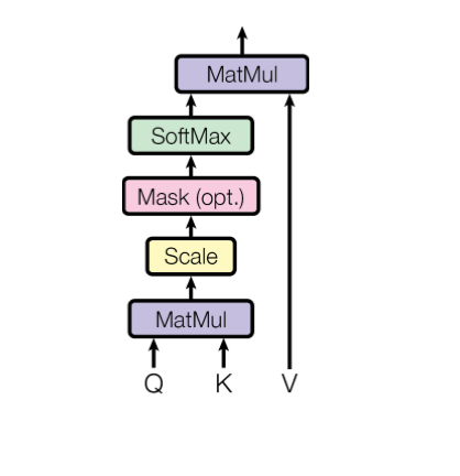
Attention可以看成一个函数,它的输入是Query,Key,Value和Mask,输出是一个Tensor。其中输出是Value的加权平均,而权重来自Query和Key的计算。具体的计算如下图所示,计算公式为:
1 | def attention(query, key, value, mask=None, dropout=None): |
我们知道, 在训练的时候, 我们是以 batch_size 为单位的, 那么就会有 padding, 一般我们取 pad == 0, 那么就会造成在 Attention 的时候, query 的值为 0, query 的值为 0, 所以我们计算的对应的 scores 的值也是 0, 那么就会导致 softmax 很可能分配给该单词一个相对不是很小的比例, 因此, 我们将 pad 对应的 score 取值为负无穷(普通的计算,score可以为负数?不是,根据softmax的计算公式,就算pad=0,那么e^0=1,也是会占有一些概率值的), 以此来减小 pad 的影响.
很容易想到, 在 decoder, 未预测的单词也是用 padding 的方式加入到 batch 的, 所以使用的mask 机制与 padding 时mask 的机制是相同的, 本质上都是query 的值为0, 只是 mask 矩阵不同, 我们可以根据 decoder 部分的代码发现这一点.
我们使用一个实际的例子跟踪一些不同Tensor的shape,然后对照公式就很容易理解。比如Q是(30,8,33,64),其中30是batch,8是head个数,33是序列长度,64是每个时刻的特征数(size)。K和Q的shape必须相同的,而V可以不同,但是这里的实现shape也是相同的。
1 | scores = torch.matmul(query, key.transpose(-2, -1)) \ |
上面的代码实现 ,和公式里稍微不同的是,这里的Q和K都是4d的Tensor,包括batch和head维度。matmul会把query和key的最后两维进行矩阵乘法,这样效率更高,如果我们要用标准的矩阵(二维Tensor)乘法来实现,那么需要遍历batch维和head维:
1 | batch_num = query.size(0) # query.size(0)返回的是0维的数 |
而上面的写法一次完成所有这些循环,效率更高。输出的score是(30, 8, 33, 33),前面两维不看,那么是一个(33, 33)的attention矩阵a,aij表示时刻 i关注 j 的得分(还没有经过softmax变成概率)。
在编码器的attention中src_mask的作用!!!
接下来是scores.masked_fill(mask == 0, -1e9),用于把mask是0的变成一个很小的数,这样后面经过softmax之后的概率就很接近零(但是理论上还是用来很少一点点未来的信息)。
masked_fill_(mask, value):掩码操作 masked_fill方法有两个参数,maske和value,mask是一个pytorch张量(Tensor),元素是布尔值,value是要填充的值,填充规则是mask中取值为True位置对应于self的相应位置用value填充。
注:参数mask必须与score的size相同或者两者是可广播(broadcasting-semantics)的
pytorch masked_fill方法简单理解
https://blog.csdn.net/jianyingyao7658/article/details/103382654
pytorch 广播语义(Broadcasting semantics)
https://blog.csdn.net/qq_35012749/article/details/88308657
这里mask是(30, 1, 1, 33)的tensor,因为8个head的mask都是一样的,所有第二维是1,masked_fill时使用broadcasting就可以了。这里是self-attention的mask,所以每个时刻都可以attend到所有其它时刻,所有第三维也是1,也使用broadcasting。如果是普通的mask,那么mask的shape是(30, 1, 33, 33)。
这样讲有点抽象,我们可以举一个例子,为了简单,我们假设batch=2, head=8。第一个序列长度为3,第二个为4,那么self-attention的mask为(2, 1, 1, 4),我们可以用两个向量表示:
1 | 1 1 1 0 |
它的意思是在self-attention里,第一个序列的任一时刻可以attend to 前3个时刻(因为第4个时刻是padding的);而第二个序列的可以attend to所有时刻的输入。而Decoder的src-attention的mask为(2, 1, 4, 4),我们需要用2个矩阵表示:(一个序列对应一个一维src_mask(1×4), 一个序列对应一个二维的tgt_mask(4×4))
1 | 第一个序列的mask矩阵 |
接下来对score求softmax,把得分变成概率p_attn,如果有dropout还对p_attn进行Dropout(这也是原始论文没有的)。最后把p_attn和value相乘。p_attn是(30, 8, 33, 33),value是(30, 8, 33, 64),我们只看后两维,(33x33) x (33x64)最终得到33x64。
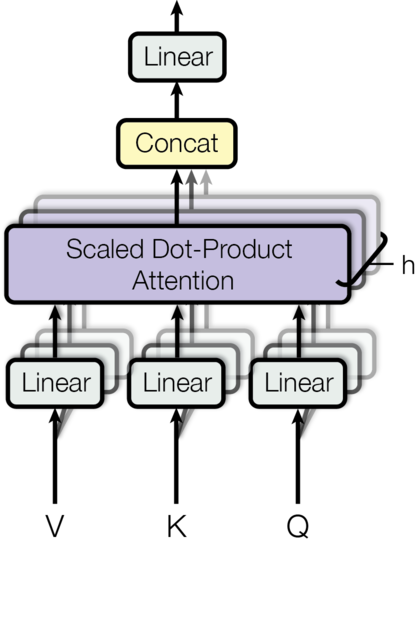
接下来就是输入怎么变成Q,K和V了,对于每一个Head,都使用三个矩阵WQ,WK,WV把输入转换成Q,K和V。然后分别用每一个Head进行Self-Attention的计算,最后把N个Head的输出拼接起来,最后用一个矩阵WO把输出压缩一下。具体计算过程为:
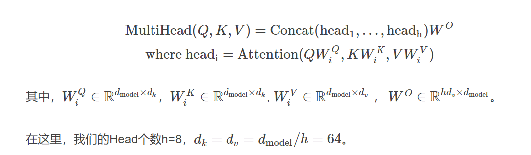
详细结构如下图所示,输入Q,K和V经过多个线性变换后得到N(8)组Query,Key和Value,然后使用Self-Attention计算得到N个向量,然后拼接起来,最后使用一个线性变换进行降维。
1 | class MultiHeadedAttention(nn.Module): |
我们先看构造函数,这里d_model(512)是Multi-Head的输出大小,因为有h(8)个head,因此每个head的d_k=512/8=64。接着我们构造4个(d_model , d_model)的矩阵,后面我们会看到它的用处。最后是构造一个Dropout层。
然后我们来看forward方法。输入的mask是(batch, 1, time)的,因为每个head的mask都是一样的,所以先用unsqueeze(1)变成(batch, 1, 1, time),mask我们前面已经详细分析过了。
接下来是根据输入query,key和value计算变换后的Multi-Head的query,key和value。这是通过下面的语句来实现的:
1 | query, key, value = \ |
zip(self.linears, (query, key, value))是把(self.linears[0],self.linears[1],self.linears[2])和(query, key, value)放到一起然后遍历。我们只看一个self.linears[0] (query)。根据构造函数的定义,self.linears[0]是一个(512, 512)的矩阵,而query是(batch, time, 512),相乘之后得到的新query还是512(d_model)维的向量,然后用view把它变成(batch, time, 8, 64)。然后transponse成(batch, 8,time,64),这是attention函数要求的shape。分别对应8个Head,每个Head的Query都是64维。
1.一般来说,矩阵相乘,[a,b] x [b,c] = [a,c]
所以不同维度要进行处理,必须降维。
例如 A 矩阵 [a,b,c], B 矩阵是[c,d],这个时候就需要将 A 矩阵看成是 [axb, c] 与 [c,d] 进行相乘,得到结果。
- Linear函数l(x),应该就是 (batch*time,512)**(512,512)
Key和Value的运算完全相同,因此我们也分别得到8个Head的64维的Key和64维的Value。接下来调用attention函数,得到x和self.attn。其中x的shape是(batch, 8, time, 64),而attn是(batch, 8, time, time)。
time是倍数
x.transpose(1, 2)把x变成(batch, time, 8, 64),然后把它view成(batch, time, 512),其实就是把最后8个64维的向量拼接成512的向量。最后使用self.linears[-1]对x进行线性变换,self.linears[-1]是(512, 512)的,因此最终的输出还是(batch, time, 512)。我们最初构造了4个(512, 512)的矩阵,前3个用于对query,key和value进行变换,而最后一个对8个head拼接后的向量再做一次变换。
Attention在模型中的应用
在Transformer里,有3个地方用到了MultiHeadedAttention:
Encoder的Self-Attention层
query,key和value都是相同的值,来自下层的输入。Mask都是1(当然padding的不算)。
Decoder的Self-Attention层
query,key和value都是相同的值,来自下层的输入。但是Mask使得它不能访问未来的输入。
Encoder-Decoder的普通Attention
query来自下层的输入,而key和value相同,是Encoder最后一层的输出,而Mask都是1。
Position-wise 前馈网络
In addition to attention sub-layers, each of the layers in our encoder and decoder contains a fully connected feed-forward network, which is applied to each position separately and identically. This consists of two linear transformations with a ReLU activation in between.
全连接层有两个线性变换以及它们之间的ReLU激活组成:

全连接层的输入和输出都是d_model(512)维的,中间隐单元的个数是d_ff(2048)维
1 | class PositionwiseFeedForward(nn.Module): |
Embeddings 和 Softmax
输入的词序列都是ID序列,我们需要Embedding。源语言和目标语言都需要Embedding,此外我们需要一个线性变换把隐变量变成输出概率,这可以通过前面的类Generator来实现。我们这里实现Embedding:
1 | class Embeddings(nn.Module): |
注意的就是forward处理使用nn.Embedding对输入x进行Embedding之外,还除以了sqrt(d_model) (开方)
位置编码
位置编码的公式为:
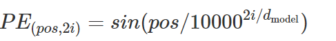
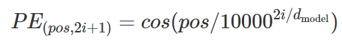
where pos is the position and i is the dimension. That is, each dimension of the positional encoding corresponds to a sinusoid.
假设输入是ID序列长度为10,如果输入Embedding之后是(10, 512),那么位置编码的输出也是(10, 512)。上式中pos就是位置(0-9),512维的偶数维使用sin函数,而奇数维使用cos函数。这种位置编码的好处是:PE_pos+k可以表示成 PE_pos的线性函数,这样网络就能容易的学到相对位置的关系。
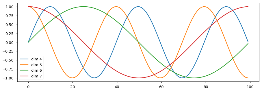
1 | plt.figure(figsize=(15, 5)) |
图是一个示例,向量的大小d_model=20,我们这里画出来第4、5、6和7维(下标从零开始)维的图像,最大的位置是100。我们可以看到它们都是正弦(余弦)函数,而且周期越来越长。
前面我们提到位置编码的好处是PE_pos+k可以表示成 P_Epos的线性函数,我们下面简单的验证一下。我们以第i维为例,为了简单,我们把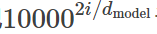 记作Wi,这是一个常量。
我们发现PE_pos+k 确实可以表示成 PE_pos的线性函数。
In addition, we apply dropout to the sums of the embeddings and the positional encodings in both the encoder and decoder stacks. For the base model, we use a rate of Pdrop=0.1.
1 | class PositionalEncoding(nn.Module): |
代码可以参考公式,调用了Module.register_buffer函数。这个函数的作用是创建一个buffer,比如这里把pe保存下来。register_buffer通常用于保存一些模型参数之外的值,比如在BatchNorm中,我们需要保存running_mean(Moving Average),它不是模型的参数(不用梯度下降),但是模型会修改它,而且在预测的时候也要使用它。这里也是类似的,pe是一个提前计算好的常量,我们在forward要用到它。我们在构造函数里并没有把pe保存到self里,但是在forward的时候我们却可以直接使用它(self.pe)。如果我们保存(序列化)模型到磁盘的话,PyTorch框架也会帮我们保存buffer里的数据到磁盘,这样反序列化的时候能恢复它们
完整模型
Here we
define a function that takes in hyperparameters and produces a full model.
1 |
|
首先把copy.deepcopy命名为c,这样使下面的代码简洁一点。然后构造MultiHeadedAttention,PositionwiseFeedForward和PositionalEncoding对象。接着就是构造EncoderDecoder对象。它需要5个参数:Encoder、Decoder、src-embed、tgt-embed和Generator。
我们先看后面三个简单的参数,Generator直接构造就行了,它的作用是把模型的隐单元变成输出词的概率。而src-embed是一个Embeddings层和一个位置编码层c(position),tgt-embed也是类似的。
最后我们来看Decoder(Encoder和Decoder类似的)。Decoder由N个DecoderLayer组成,而DecoderLayer需要传入self-attn, src-attn,全连接层和Dropout。因为所有的MultiHeadedAttention都是一样的,因此我们直接deepcopy就行;同理所有的PositionwiseFeedForward也是一样的网络结果,我们可以deepcopy而不要再构造一个。
训练
This section describes the training regime for our models.
We stop for a quick interlude to introduce some of the tools needed to train a standard encoder decoder model. First
we define a batch object that holds the src and target sentences for training, as well as constructing the masks.
Batches 和 Masking
mask 矩阵来自 batch
self.src_mask = (src != pad).unsqueeze(-2) 也就是说, 源语言的 mask 矩阵的维度是 (batch_size, 1, length), 那么为什么 attn_shape = (batch_size, size, size) 呢? 可以这么解释, 在 encoder 阶段的 Self_Attention 阶段, 所有的 Attention 是可以同时进行的, 把所有的 Attention_result 算出来, 然后用同一个 mask vector * Attention_result 就可以了, 但是在 decoder 阶段却不能这么做, 我们需要关注的问题是:
根据已经预测出来的单词预测下面的单词, 这一过程是序列的,
而我们的计算是并行的, 所以这一过程中, 必须要引入矩阵. 也就是上面的 subsequent_mask() 函数获得的矩阵.
这个矩阵也很形象, 分别表示已经预测的单词的个数为, 1, 2, 3, 4, 5.
然后我们将以上过程反过来过一篇, 就很明显了, 在batch阶段获得 mask 矩阵, 然后和 batch 一起训练, 在 encoder 与 deocder 阶段实现 mask 机制.
mask在Batch中定义,src_mask.size (30,1,10) , trg_mask.size(30,10,10)
然后在MultiHeadedAttention中
mask = mask.unsqueeze(1)又扩维了,其中src_mask.size(30,1,1,10) ,trg_mask.size(30,1,10,10)
src_mask.size满足attention中的维度,所以可以对score进行mask
src_mask还在解码器的第1子层用到,相同的原理
trg_mask在解码器的第0子层用到,满足要求
1 | class Batch: #定义每一个batch中的src、tgt、mask |
Batch构造函数的输入是src和trg,后者可以为None,因为再预测的时候是没有tgt的。
我们用一个例子来说明Batch的代码,这是训练阶段的一个Batch,src是(48, 20),48是batch大小,而20是最长的句子长度,其它的不够长的都padding成20了。而trg是(48, 25),表示翻译后的最长句子是25个词,不足的也padding过了。
我们首先看src_mask怎么得到,(src != pad)把src中大于0的时刻置为1,这样表示它可以attend to的范围。然后unsqueeze(-2)把src_mask变成(48/batch, 1, 20/time)。它的用法参考前面的attention函数。
对于训练来说(Teaching Forcing模式),Decoder有一个输入和一个输出。比如句子”
注意src_mask的shape是(batch, 1, time),而trg_mask是(batch, time, time)。因为src_mask的每一个时刻都能attend to所有时刻(padding的除外),一次只需要一个向量就行了,而trg_mask需要一个矩阵。
Training Loop
1 | def run_epoch(data_iter, model, loss_compute): #返回total_loss / total_tokens 。是一个数值,损失计算 |
它遍历一个epoch的数据,然后调用forward,接着用loss_compute函数计算梯度,更新参数并且返回loss。这里的loss_compute是一个函数,它的输入是模型的预测out,真实的标签序列batch.trg_y和batch的词个数。实际的实现是MultiGPULossCompute类,这是一个callable。本来计算损失和更新参数比较简单,但是这里为了实现多GPU的训练,这个类就比较复杂了。
Training Data 和 Batching
We trained on the standard WMT 2014 English-German dataset consisting of about 4.5 million sentence pairs. Sentences were encoded using byte-pair encoding, which has a shared source-target vocabulary of about 37000 tokens. For English- French, we used the significantly larger WMT 2014 English-French dataset consisting of 36M sentences and split tokens into a 32000 word-piece vocabulary.
Sentence pairs were batched together by approximate sequence length. Each training batch contained a set of sentence pairs containing approximately 25000 source tokens and 25000 target tokens.
We will use torch text for batching. This is discussed in more detail below. Here we create batches in a torchtext function that ensures our batch size padded to the maximum batchsize does not surpass a threshold (25000 if we have 8 gpus).
1 | global max_src_in_batch, max_tgt_in_batch |
硬件 和 训练进度
We trained our models on one machine with 8 NVIDIA P100 GPUs. For our base models using the hyperparameters described throughout the paper, each training step took about 0.4 seconds. We trained the base models for a total of 100,000 steps or 12 hours. For our big models, step time was 1.0 seconds. The big models were trained for 300,000 steps (3.5 days).
Optimizer
We used the Adam optimizer (cite) with β1=0.9β1=0.9, β2=0.98β2=0.98 and ϵ=10−9ϵ=10−9. We varied the learning rate over the course of training, according to the formula: lrate=d−0.5model⋅min(step_num−0.5,step_num⋅warmup_steps−1.5)lrate=dmodel−0.5⋅min(step_num−0.5,step_num⋅warmup_steps−1.5) This corresponds to increasing the learning rate linearly for the first warmupstepswarmupsteps training steps, and decreasing it thereafter proportionally to the inverse square root of the step number. We used warmupsteps=4000warmupsteps=4000.
Note: This part is very important. Need to train with this setup of the model.
1 | class NoamOpt: |
Example of the curves of this model for different model sizes and for optimization hyperparameters.
1 | # Three settings of the lrate hyperparameters. |
![]()
Regularization
Label Smoothing
During training, we employed label smoothing of value ϵls=0.1ϵls=0.1 (cite). This hurts perplexity, as the model learns to be more unsure, but improves accuracy and BLEU score.
We implement label smoothing using the KL div loss. Instead of using a one-hot target distribution, we create a distribution that has
confidenceof the correct word and the rest of thesmoothingmass distributed throughout the vocabulary.
1 | class LabelSmoothing(nn.Module): |
Here we can see an example of how the mass is distributed to the words based on confidence.
1 | # Example of label smoothing. |
![]()
Label smoothing actually starts to penalize the model if it gets very confident about a given choice.
1 | crit = LabelSmoothing(5, 0, 0.1) |
![]()
总结
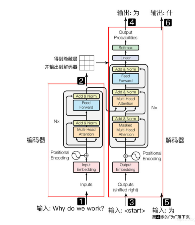
transformer模型主要分为两大部分, 分别是编码器和解码器, 编码器负责把自然语言序列映射成为隐藏层(下图中第2步用九宫格比喻的部分), 含有自然语言序列的数学表达. 然后解码器把隐藏层再映射为自然语言序列, 从而使我们可以解决各种问题, 如情感分类, 命名实体识别, 语义关系抽取, 摘要生成, 机器翻译等等, 下面我们简单说一下下图的每一步都做了什么:
1.输入自然语言序列到编码器: Why do we work?(为什么要工作);
2.编码器输出的隐藏层, 再输入到解码器;
3.输入<𝑠𝑡𝑎𝑟𝑡>
(起始)符号到解码器; 4.得到第一个字"为";
5.将得到的第一个字"为"落下来再输入到解码器;
6.得到第二个字"什";
7.将得到的第二字再落下来, 直到解码器输出<𝑒𝑛𝑑>
(终止符), 即序列生成完成.
原始data数据是:(30,10)
src: (30,10) trg:(30,10)
在encoder中,
embedding: 参数x就是 src (30,10) 经过处理之后, x:(30,10,512)
-> 即输入给encoder的x:(30,10,512)
经过encoder各个层处理之后,输出的(30,10,512) memory是encoder的输出,但是为什么memory:(1,10,512) ??? 因为在预测时 ,src是(1,10),不是(30,10)所以memory是(1,10,512)
decoder中:输入来自 memory 和 trg_emd
embedding : 参数x是trg(30,9),经过处理之后,x:(30,9,512)
经过decoder各个层处理之后,输出的(30,9 , 512)
再经过generator层之后,x:(30,9,11)
在预测的时候是(1,1,512),不是(1,9,512),在预测完generator之后,(1,11),选一个最大的。
因为是一个数字一个数字预测输出的,所以是1,不是9
具体流程
transformer的encoder部分,是并行计算各个token之间的关系,然后输出给decoder一个memory,decoder再产生预测值,计算loss之后,再反向传播。因为是一个计算图,所以encoder和decoder的参数都会更新。
参数更新完之后,下一个batch的数据再输进来,再计算loss,再更新,以此循环
第一个例子
We can begin by trying out a simple copy-task. Given a random set of input symbols from a small vocabulary, the goal is to generate back those same symbols.
Synthetic Data
1 | def data_gen(V, batch, nbatches): # batch=30:一次输入多少, nbatch=20:输入多少次 |
Loss Computation
1 | class SimpleLossCompute: #loss计算以及更新。调用LabelSmoothing,使用KL散度 |
Greedy Decoding
1 | # Train the simple copy task. |
This code predicts a translation using greedy decoding for simplicity.
1 | #预测过程 |
真实例子
Now we consider a real-world example using the IWSLT German-English Translation task. This task is much smaller than the WMT task considered in the paper, but it illustrates the whole system. We also show how to use multi-gpu processing to make it really fast.
1 | #!pip install torchtext spacy |
Data Loading
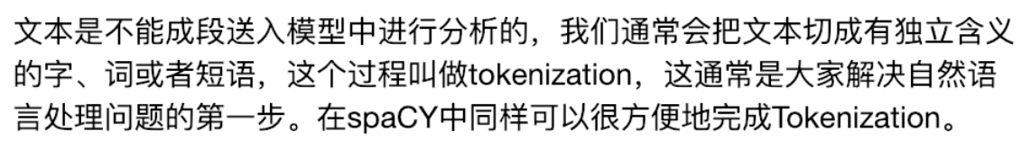
We will load the dataset using torchtext and spacy for tokenization.
用torchtext来加载数据集 , 用spacy来分词
torchtext组件流程:
- 定义Field:声明如何处理数据,主要包含以下数据预处理的配置信息,比如指定分词方法,是否转成小写,起始字符,结束字符,补全字符以及词典等等
- 定义Dataset:用于得到数据集,继承自pytorch的Dataset。此时数据集里每一个样本是一个 经过 Field声明的预处理 预处理后的 wordlist
- 建立vocab:在这一步建立词汇表,词向量(word embeddings)
- 构造迭代器Iterator:: 主要是数据输出的模型的迭代器。构造迭代器,支持batch定制用来分批次训练模型。
1 | # For data loading. |
批训练对于速度来说很重要。希望批次分割非常均匀并且填充最少。 要做到这一点,我们必须修改torchtext默认的批处理函数。 这部分代码修补其默认批处理函数,以确保我们搜索足够多的句子以构建紧密批处理。 一般来说直接调用
BucketIterator(训练用)和Iterator(测试用) 即可
BucketIterator和Iterator的区别是,BucketIterator尽可能的把长度相似的句子放在一个batch里面。
Iterators
1 | """ |
Multi-GPU Training
最后为了真正地快速训练,将使用多个GPU。 这部分代码实现了多GPU字生成,它不是Transformer特有的。 其思想是将训练时的单词生成分成块,以便在许多不同的GPU上并行处理。 我们使用PyTorch并行原语来做到这一点:
- replicate -复制 - 将模块拆分到不同的GPU上
- scatter -分散 - 将批次拆分到不同的GPU上
- parallel_apply -并行应用 - 在不同GPU上将模块应用于批处理
- gather - 聚集 - 将分散的数据聚集到一个GPU上
- nn.DataParallel - 一个特殊的模块包装器,在评估之前调用它们。
1 | # Skip if not interested in multigpu. |
Now we create our model, criterion, optimizer, data iterators, and paralelization
1 | # GPUs to use |
Now we train the model. I will play with the warmup steps a bit, but everything else uses the default parameters. On an AWS p3.8xlarge with 4 Tesla V100s, this runs at ~27,000 tokens per second with a batch size of 12,000
在具有4个Tesla V100 GPU的AWS p3.8xlarge机器上,每秒运行约27,000个词,批训练大小为12,000。
Training the System
1 | #!wget https://s3.amazonaws.com/opennmt-models/iwslt.pt |
Once trained we can decode the model to produce a set of translations. Here we simply translate the first sentence in the validation set. This dataset is pretty small so the translations with greedy search are reasonably accurate.
1 | #类比于run_epoch函数 |
理解QKV
作者:繁华里流浪 链接:https://www.zhihu.com/question/298810062/answer/1336554776 来源:知乎 著作权归作者所有。商业转载请联系作者获得授权,非商业转载请注明出处。
我认为attention主要分为两个核心步骤:1. 计算注意力权重 2. 加权求和
其中Q(query),K(key)用来计算对应的注意力权重atten_i,V(value)用来进行加权求和也就是求最后attention的结果。

在理解attention的时候我想了一个买水果的例子。今天你要去水果摊买水果,首先你脑袋里会想出一个买水果的标准(个大、成色好、价格美丽等)作为 query,然后你就去各个水果摊逛了,水果摊主上来给你拿出水果一顿介绍(我这香甜可口,新鲜美味,性价比高)这就是 key,然后你会通过水果的情况 key 和自己心中标准 query 权衡给这个水果摊子打个分,当你一条水果街都走完了,你就对整条街的水果摊都有了一个性价比分数(atten),然后根据这个性价比分数就开始买了,这个水果摊好分数高,我买多点,那个水果摊性价比分数低不能满足我的需求我就少买点,最后我就从不同的水果摊采购了不同数量的水果(value)放进了自己的推推车里(output)